Experiment 4: Conservation of Energy

(Also look over lab 5 today: You need to collect some information ahead of time, which you should start planning now.)

OBJECT: To verify that energy is conserved as a glider moves on an air track.

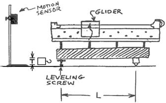APPARATUS: Compressed air blows out of holes on the air track, lifting the glider off its surface, so that its motion is virtually frictionless. The glider's position is recorded periodically using a computerized sensor, which sends out pulses of ultrasound and measuring the time for echoes to return. From how the glider's position changes with time, the computer can calculate velocity, as you did by hand in the freefall lab.

PROCEDURE:

1. Check that the power strip is plugged in, then turn on its switch. This should turn on both the computer and interface.

2. Measure the mass of the glider using a balance. Measure L, the distance between the track's feet. (See picture) Measure T, the thickness of the metal block to the nearest millimeter or better.

3. Place the air track (and sensor) as close to the outside edge of the counter as you can get it. This is to avoid echoes from the shelf at the counter's center, and the things around it.

4. Put the sensor in line with the air track, about a foot beyond the end supported by one screw. Move the air track, if necessary, to make room for it. The bottom of the round shiny part of the sensor should be about 44 or 45 cm above the counter.

5. Level the air track: With the air on, adjust its screw-in foot so that a glider placed at rest will not coast either way. (It will always move a little after you let go of it, but there should be no consistent direction that it goes when released from various points. If the track seems to badly need straightening, inform the instructor.) Once level, do not move the air track, or you might unlevel it again.

6. Check for friction: After a gentle nudge, the glider should creep from one end to the other without noticeably slowing down. Once level, you can turn the air off for a while.

7. Insert the metal block under the track's leveling screw (not the end with two screws) to tilt the track.

8. Get the computer ready: Click on Science Workshop, then in the window which appears, double click on Science Workshop. A kindly physics instructor has already set up the sensors and graph for you. To retrieve this, click on file, then on open, then on the file called 100lab4.sws, then on ok.

9. Aim the motion sensor: Measure how far the glider is from the sensor, using a meterstick. Then, double click on the picture of the motion sensor, just below the picture of the interface box. In the window that appears, watch "current distance" near the upper left as you twist the sensor about a horizontal axis: Starting with it aimed too high, turn it down until the distance matches what you measured. Don't aim it any lower than necessary. Move the glider around the track by hand to make sure the distance changes along with it. Don't worry if it doesn't see the glider for a small part of the track near one end. Click ok.

10. Hold the glider near the upper end of the track. Click on REC at the upper left. When REC gets fainter, after a couple of seconds, release the glider. When it gets to the other end of the track, click STOP. While the sensor is running, keep anything which might reflect ultrasound, such as your hands, out of the general area so it doesn't watch the wrong object.

ANALYSIS OF DATA

1. Display the glider's velocity versus position on a graph:

a. Double click on "graph display" at the lower left. The data is probably crowded into a small part of the graph. Change scales to get a better look it: One way to do this is with the + and - buttons at the lower right. Another way which is sometimes easier is to use the magnifier: Click this button: Then, click at one corner of the area you want to see, and release the button at the opposite corner. The area you outlined will then be magnified to fill the entire graph.

b. Is it a good run? The beginning and end of the graph probably look pretty messy, with a fairly straight part in between. If the straight part isn't at least 50 cm long, ask the instructor to help aim the sensor better, and try again. The new data will automatically load into the graph.

c. Best fit curve: The graph includes a curve which averages out the random jumps in the data. To tell it which points to fit to and which to ignore, use the mouse to draw a box around the good ones, highlighting them.

2. From the best fit curve, read the velocity and position of the glider at a point near the beginning of the graph. Repeat at a point near the end, at least 50 cm away. (Farther is better.) To read these, click on this ; the coordinates where the pointer is located will then appear next to the axes of the graph. Don’t turn off the computer until the instructor accepts your paper, in case your data needs to be rechecked.

1

3. Find the distance, d, between these points by subtracting.

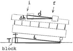
4. Find the vertical distance, Δh, which the glider moves between points i and f. This is not just the thickness of the block, because the distance the glider moved between i and f is not the same as the distance between the air track's feet. Rather, notice that the two highlighted triangles are the same shape ("similar triangles"), and therefore should have the same ratio between their sides:

Δh/d = T/L. Solving this for Δh,

Δh = d(T/L)

5. Before doing the rest of this, convert grams to kilograms and centimeters to meters, because these are the units which the joule is based on. Otherwise, you will make a decimal error. (What units you used before this point doesn't matter.)

6. How many joules did the glider's potential energy change between points i and f? Since potential energy equals mgh, the change in potential energy is mg times the change in height, mgΔh.

7. How many joules did the glider's kinetic energy change between points i and f? It's a little trickier than with potential energy, because the speed is squared: Find its kinetic energy at point f, find its kinetic energy at point i, then subtract.

8. Conclusion: Compare the potential energy lost to the kinetic energy gained. Does the total seem to be staying about the same?

Again, be sure to look over lab 5 now also. At the start of the period, you will need:

1. The weight of the car (printed on the registration).

2. Its gas mileage.

3. The results of the road test.

Experiment #4: Conservation of Energy

Name _________________________________

glider's mass = _____________________

L = _____________________ T = _____________________

INITIALLY:

x = _____________________ v_i = _____________________

FINALLY:

x = _____________________ v_f = _____________________

d = _____________________

Compute Δh :

Compute ΔPE :

Compute ΔKE :

Conclusion: